Parametric approach to visualize parabolic trajectories
Join me with a Python-based project that helps visualize parabolic trajectories with user-defined impact points and maximum heights. We’ll talk about the underlying math, parametric equations, and visualization techniques to enhance your understanding of parabolic motion.
Visualizing a Parabola with a Given Impact Point
In this blog post, we will explore a project that calculates the parametric equation of a parabola and visualizes it in three-dimensional space, given a user-defined impact point and maximum height. We will begin with a brief introduction to the mathematics behind the problem and then delve into the details of the project.
Mathematical Background
The problem we are trying to solve involves finding a parabolic trajectory that passes through an origin , reaches a given maximum height , and lands at a user-defined impact point . To do this, we will use parametric equations to describe the parabola in three-dimensional space. These equations are as follows:
Where is the parameter that varies along the trajectory.
We know three points on our parabola: the origin , the maximum point , and the impact point . Using these points, we can set up a system of linear equations for each dimension to solve for the coefficients , , , , , , , , and .
Once we have these coefficients, we can construct the parametric equation of the parabolic trajectory as follows:
Which can be rewritten as:
This equation can be directly inputted into graphing software like GeoGebra (or similar) to visualize the trajectory and manipulate it dynamically:
(at^2 + bt + c, dt^2 + et + f, gt^2 + ht + i)
Project Overview
The project takes a user-defined impact point and the maximum height (), calculates the parametric equation describing the parabola, and then visualizes the resulting graph in three-dimensional space.
Technologies
- Python
- Libraries:
matplotlibnumpy
Dependencies
To install the dependencies:
$ pip install -r requirements.txt
Execution
To run the program:
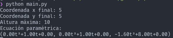
$ python main.py
Users will need to input the following data:
- coordinate of the impact point: any real number.
- coordinate of the impact point: any real number.
- Maximum height () of the parabolic trajectory.
Source code
1 2 3 4 5 6 7 8 9 10 11 12 13 14 15 16 17 18 19 20 21 22 23 24 25 26 27 28 29 30 31 32 33 34 35 36 37 38 39 40 41 42 43 44 45 46 47 48 49 50 51 52 53 54 55 56 57 58 59 60 61 62 63 64 65 66 67 68 69 70 71 72 73 74 75 76 77 78 79 80 81 82 83 84 85 86 87 88 89 90 91 92 | import matplotlib.pyplot as plt import numpy as np # Entradas del usuario. xf = float(input("Coordenada x final: ")) yf = float(input("Coordenada y final: ")) hmax = float(input("Altura máxima: ")) # Planteamiento de matrices del sistema de ecuaciones lineales. primerMatriz = np.array([ [0, 0, 1], [(xf/2)**2, xf/2, 1], [xf**2, xf, 1] ]) segundaMatriz = np.array([ [0, 0, 1], [(xf/2)**2, xf/2, 1], [xf**2, xf, 1] ]) tercerMatriz = np.array([ [0, 0, 1], [(xf/2)**2, xf/2, 1], [xf**2, xf, 1] ]) # Términos independientes para nuestro sistema de ecuaciones lineales. terminosIndependientes1 = np.array([0, xf/2, xf]) terminosIndependientes2 = np.array([0, yf/2, yf]) terminosIndependientes3 = np.array([0, hmax, 0]) # Cálculo de las soluciones de los sistemas 3x3 solucionesX = np.linalg.solve(primerMatriz, terminosIndependientes1) solucionesY = np.linalg.solve(segundaMatriz, terminosIndependientes2) solucionesZ = np.linalg.solve(tercerMatriz, terminosIndependientes3) # Imprimir en la terminal la ecuación paramétrica de la parábola resultante. print("Ecuación paramétrica:") print(f"({solucionesX[0]:.2f}t²+{solucionesX[1]:.2f}t+{solucionesX[2]:.2f}, {solucionesY[0]:.2f}t²+{solucionesY[1]:.2f}t+{solucionesY[2]:.2f}, {solucionesZ[0]:.2f}t²+{solucionesZ[1]:.2f}t+{solucionesZ[2]:.2f})") # Creamos la figura de Matplotlib fig = plt.figure() # Creamos la gráfica ax = fig.add_subplot(projection='3d') # Creamos los ejes. xx, yy = np.meshgrid(range(20), range(20)) # Creamos el rango de valores para t t_line = np.linspace(0, 10, 100) # Planteamos las ecuaciones paramétricas en función de t x_line = (solucionesX[0] * (t_line ** 2)) + \ (solucionesX[1] * t_line) + solucionesX[2] y_line = (solucionesY[0] * (t_line ** 2)) + \ (solucionesY[1] * t_line) + solucionesY[2] z_line = (solucionesZ[0] * (t_line ** 2)) + \ (solucionesZ[1] * t_line) + solucionesZ[2] # Añadimos el punto de impacto punto = ax.plot([xf], [yf], [0], markerfacecolor='k', markeredgecolor='k', marker='o', markersize=5, alpha=0.6) # Añadimos las ecuaciones paramétricas a nuestra gráfica en 3D curva = ax.plot3D(x_line, y_line, z_line, label='Curva Paramétrica', color="red") # Colocamos los límites de graficación en los ejes. ax.set_xlim(-1, 15) ax.set_ylim(-1, 15) ax.set_zlim(-1, 15) # Colocamos las etiquetas en los ejes. ax.set_xlabel('x', color='blue') ax.set_ylabel('y', color='blue') ax.set_zlabel('z', color='blue') # Colocamos el título de la gráfica ax.set_title("Curva Paramétrica de Tiro Parabólico") # Proxies para colores de la leyenda. proxy_grafica = plt.Rectangle((0, 0), 1, 1, fc='r') proxy_punto = plt.Line2D( [0], [0], linestyle="none", marker='o', alpha=0.6, markersize=10, markerfacecolor='black') # Mostrar la leyenda ax.legend([proxy_grafica, proxy_punto], [f"({solucionesX[0]:.2f}t²+{solucionesX[1]:.2f}t+{solucionesX[2]:.2f}, {solucionesY[0]:.2f}t²+{solucionesY[1]:.2f}t+{solucionesY[2]:.2f}, {solucionesZ[0]:.2f}t²+{solucionesZ[1]:.2f}t+{solucionesZ[2]:.2f})", f"Impacto ({xf:.2f},{yf:.2f},0)"], numpoints=1, loc='lower left') # Mostramos la gráfica plt.show() |
Credits
This program was created for the Vector Analysis course at the Escuela Superior de Cómputo of the Instituto Politécnico Nacional, taught by Dr. Dárwin Gutiérrez Mejía.
May 2021
Note from 2023.
This project was written in May 2021, however I never had the time to get to write a little about it. If you’re curious about the code and/or the original written report (which is basically the spanish version of what you just read) you can find it here:
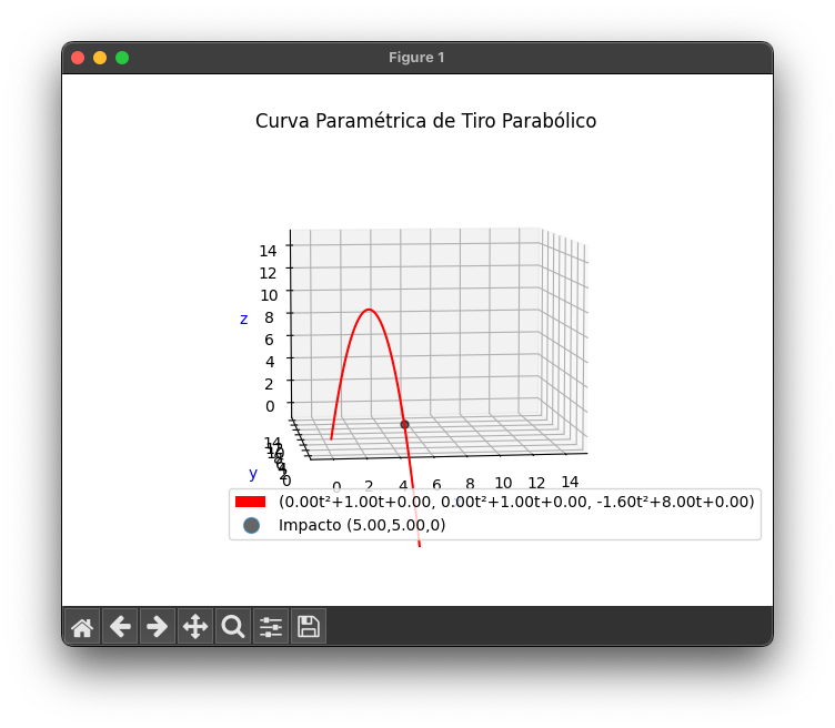
If you run the code with the following command:
The output will be something like these options:
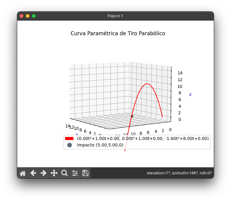
Thank you for reading! I hope you can find some inspiration here to make some cool visualizations for your classes.